|

 content.")
Cumulative Distribution Function
The Cumulative Distribution Function (CDF) of a continuous random variable, x, is equal to the integral of its probability density function (PDF) to the left of x. This value represents the area below the PDF to the left of the point of interest, x.


X-axis: represents z-scores of measurement
Y-axis: represents the probability (cdf) of "x" or lower occurring. The range is 0-1 with 1 representing 100% of the values of "x".
A y-value of 0.5 is at the mean "x" value.
The CDF is a graphical display of the total % of results below a specific measurement. Histograms and PDF show the probabilities over a range of values.
EXAMPLE:
If the PDF of a continuous random variable is known to be 0.08x where x is valid from 0 to 5. Find the probability (cumulative distribution function) of x being less or equal to 2.3.
The PDF is given as:
f(x)=0.08x, 0 ≤ x ≤ 5
Outside this interval from 0 to 5, the PDF is zero, meaning the random variable ( X ) only takes values between 0 and 5.
The PDF describes the relative likelihood of X taking a particular value. For a continuous random variable, the probability of X being exactly equal to a specific value is zero, so probabilities are computed over intervals using integrals.
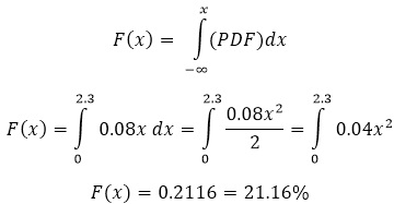
The probability P(X ≤ 2.3) is 0.2116 which means there is a 21.16% chance that x ≤ 2.3.
Inverse CDF
The inverse cumulative distribution function is used to estimate X where a certain percent of probability has occurred. If you know the cumulative area under the curve (the CDF) and you want the x-value, use the Inverse CDF.
Such as in the example above, the CDF is 21.16%. Use the inverse CDF to find that the value of x would be equal to 2.3.
Normal CDF in Excel
The function NORM.DIST (former Excel version used NORMDIST) calculates the Normal Probability Density Function or the Cumulative Normal Distribution Function.
With "x" as the point of interest, the format of the function is:
NORMDIST(x, mean, standard deviation, TRUE or FALSE)
In the final argument use:
- TRUE for the Cumulative Normal Distribution Function, or
- FALSE for the Normal Probability Density Function.
CDF calculation in Excel
Usually you will have a set of data from which you can calculate the CDF. Verify the response data is normal and determine the mean and standard deviation.
Lets assume the
Mean = 12.5
Standard Deviation = 0.25
and you want to find the CDF at x = 12.65.
Use the formula shown below.

The CDF = 72.6%
If you had the CDF value of 72.6%, you could use the inverse function in Excel
=NORM.INV(0.725747,12.5,0.25)
The answer is 12.65
EDF and CDF
An empirical cumulative distribution, aka empirical cumulative distribution function, of the same data above is shown below by gender.
This cumulative distribution function (CDF) is a step function (look closely and notice the blue lines in each chart) that jumps up by 1/n at each of the n data points. Its value at any specified value of the measured variable is the fraction of observations of the measured variable that are less than or equal to the specified value.
The empirical distribution function is an estimate of the CDF that generated the points in the sample.
The average female score is 1113 and male score is 808 which a much tighter spread (lower standard deviation) in female scores.

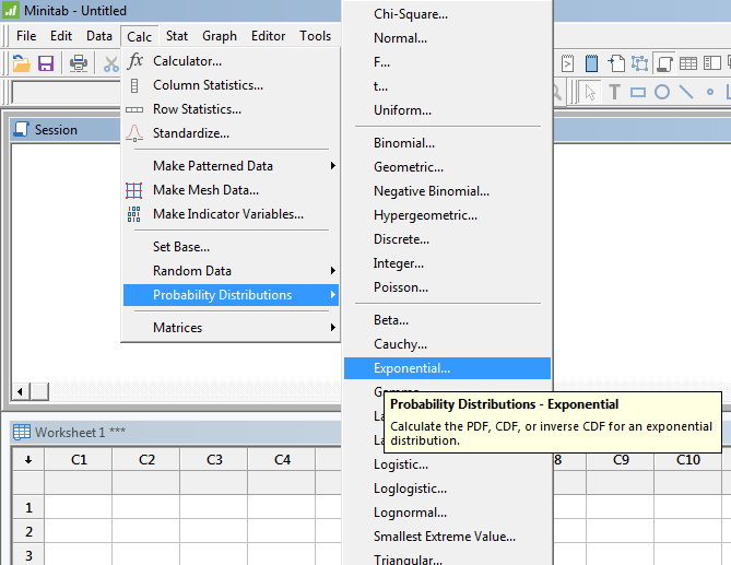
Finding Probability Distributions in Minitab
You can find the PDF, CDF, and Inverse CDF for several types of distributions. Shown below is a snapshot of the menus.
Go to the Probability Density Function (PDF)
Return to the Six-Sigma-Material Home page
Recent Articles
-
Process Capability Indices
Oct 18, 21 09:32 AM
 Determing the process capability indices, Pp, Ppk, Cp, Cpk, Cpm
 -
Six Sigma Calculator, Statistics Tables, and Six Sigma Templates
Sep 14, 21 09:19 AM
 Six Sigma Calculators, Statistics Tables, and Six Sigma Templates to make your job easier as a Six Sigma Project Manager
 -
Six Sigma Templates, Statistics Tables, and Six Sigma Calculators
Aug 16, 21 01:25 PM
Six Sigma Templates, Tables, and Calculators. MTBF, MTTR, A3, EOQ, 5S, 5 WHY, DPMO, FMEA, SIPOC, RTY, DMAIC Contract, OEE, Value Stream Map, Pugh Matrix
Recent Articles
-
Process Capability Indices
Oct 18, 21 09:32 AM
Determing the process capability indices, Pp, Ppk, Cp, Cpk, Cpm -
Six Sigma Calculator, Statistics Tables, and Six Sigma Templates
Sep 14, 21 09:19 AM
Six Sigma Calculators, Statistics Tables, and Six Sigma Templates to make your job easier as a Six Sigma Project Manager -
Six Sigma Templates, Statistics Tables, and Six Sigma Calculators
Aug 16, 21 01:25 PM
Six Sigma Templates, Tables, and Calculators. MTBF, MTTR, A3, EOQ, 5S, 5 WHY, DPMO, FMEA, SIPOC, RTY, DMAIC Contract, OEE, Value Stream Map, Pugh Matrix -
Six Sigma, Six Sigma Training, Courses, Calculators, Certification
Aug 15, 21 10:27 PM
 One site with the most common Six Sigma material, videos, examples, calculators, courses, and certification.

Site Membership
LEARN MORE
Six Sigma
Templates, Tables & Calculators
Six Sigma Slides
Green Belt Program (1,000+ Slides)
Basic Statistics
Cost of Quality
SPC
Process Mapping
Capability Studies
MSA
SIPOC
Cause & Effect Matrix
FMEA
Multivariate Analysis
Central Limit Theorem
Confidence Intervals
Hypothesis Testing
T Tests
1-Way ANOVA
Chi-Square
Correlation
Regression
Control Plan
Kaizen
MTBF and MTTR
Project Pitfalls
Error Proofing
Z Scores
OEE
Takt Time
Line Balancing
Yield Metrics
Sampling Methods
Data Classification
Practice Exam
... and more
Need a Gantt Chart?